Spatial Concepts<?xml:namespace prefix = o ns = “urn:schemas-microsoft-com:office:office” />
Oracle Spatial is an integrated set of functions and procedures that enables spatial
data to be stored, accessed, and analyzed quickly and efficiently in an Oracle9i
database.
Spatial data represents the essential location characteristics of real or conceptual
objects as those objects relate to the real or conceptual space in which they exist.
1.1 What Is Oracle Spatial?
Oracle Spatial, often referred to as Spatial, provides a SQL schema and functions
that facilitate the storage, retrieval, update, and query of collections of spatial
features in an Oracle9i database. Spatial consists of the following components:
A schema (MDSYS) that prescribes the storage, syntax, and semantics of
supported geometric data types
A spatial indexing mechanism
A set of operators and functions for performing area-of-interest queries, spatial
join queries, and other spatial analysis operations
Administrative utilities
The spatial component of a spatial feature is the geometric representation of its
shape in some coordinate space. This is referred to as its geometry.
1.2 Object-Relational Model
Spatial supports the object-relational model for representing geometries. The
object-relational model uses a table with a single column of MDSYS.SDO_
GEOMETRY and a single row per geometry instance. The object-relational model
corresponds to a “SQL with Geometry Types” implementation of spatial feature
tables in the OpenGIS ODBC/SQL specification for geospatial features.
The benefits provided by the object-relational model include:
n Support for many geometry types, including arcs, circles, compound polygons,
compound line strings, and optimized rectangles
n Ease of use in creating and maintaining indexes and in performing spatial
queries
n Index maintenance by the Oracle9i database server
n Geometries modeled in a single row and single column
n Optimal performance
1.3 Introduction to Spatial Data
Oracle Spatial is designed to make spatial data management easier and more
natural to users of location-enabled applications and Geographic Information
System (GIS) applications. Once this data is stored in an Oracle database, it can be
easily manipulated, retrieved, and related to all the other data stored in the
database.
A common example of spatial data can be seen in a road map. A road map is a
two-dimensional object that contains points, lines, and polygons that can represent
cities, roads, and political boundaries such as states or provinces. A road map is a
visualization of geographic information. The location of cities, roads, and political
boundaries that exist on the surface of the Earth are projected onto a
two-dimensional display or piece of paper, preserving the relative positions and
relative distances of the rendered objects.
The data that indicates the Earth location (latitude and longitude, or height and
depth) of these rendered objects is the spatial data. When the map is rendered, this
spatial data is used to project the locations of the objects on a two-dimensional piece
of paper. A GIS is often used to store, retrieve, and render this Earth-relative spatial
data.
Types of spatial data that can be stored using Spatial other than GIS data include
data from computer-aided design (CAD) and computer-aided manufacturing
(CAM) systems. Instead of operating on objects on a geographic scale, CAD/CAM
systems work on a smaller scale, such as for an automobile engine or printed circuit
boards.
The differences among these systems are only in the relative sizes of the data, not
the data’s complexity. The systems might all actually involve the same number of
data points. On a geographic scale, the location of a bridge can vary by a few tenths
of an inch without causing any noticeable problems to the road builders, whereas if
the diameter of an engine’s pistons are off by a few tenths of an inch, the engine will
not run. A printed circuit board is likely to have many thousands of objects etched
on its surface that are no bigger than the smallest detail shown on a road builder’s
blueprints.
These applications all store, retrieve, update, or query some collection of features
that have both nonspatial and spatial attributes. Examples of nonspatial attributes
are name, soil_type, landuse_classification, and part_number. The spatial attribute
is a coordinate geometry, or vector-based representation of the shape of the feature.
1.4 Geometry Types
A geometry is an ordered sequence of vertices that are connected by straight line
segments or circular arcs. The semantics of the geometry are determined by its type.
Spatial supports several primitive types and geometries composed of collections of
these types, including 2-dimensional:
n Points and point clusters
n Line strings
n n-point polygons
n Arc line strings (All arcs are generated as circular arcs.)
n Arc polygons
n Compound polygons
n Compound line strings
n Circles
n Optimized rectangles
2-dimensional points are elements composed of two ordinates, X and Y, often
corresponding to longitude and latitude. Line strings are composed of one or more
pairs of points that define line segments. Polygons are composed of connected line
strings that form a closed ring and the interior of the polygon is implied.
Self-crossing polygons are not supported, although self-crossing line strings are
supported. If a line string crosses itself, it does not become a polygon. A
self-crossing line string does not have any implied interior.
1.5 Data Model
The Spatial data model is a hierarchical structure consisting of elements, geometries,
and layers, which correspond to representations of spatial data. Layers are
composed of geometries, which in turn are made up of elements.
For example, a point might represent a building location, a line string might
represent a road or flight path, and a polygon might represent a state, city, zoning
district, or city block.
1.5.1 Element
An element is the basic building block of a geometry. The supported spatial element
types are points, line strings, and polygons. For example, elements might model
star constellations (point clusters), roads (line strings), and county boundaries
(polygons). Each coordinate in an element is stored as an X,Y pair. The exterior ring
and the interior ring of a polygon with holes are considered as two distinct elements
that together make up a complex polygon.
Point data consists of one coordinate. Line data consists of two coordinates
representing a line segment of the element. Polygon data consists of coordinate pair
values, one vertex pair for each line segment of the polygon. Coordinates are
defined in order around the polygon (counterclockwise for an exterior polygon
ring, clockwise for an interior polygon ring).
1.5.2 Geometry
A geometry (or geometry object) is the representation of a spatial feature, modeled
as an ordered set of primitive elements. A geometry can consist of a single element,
which is an instance of one of the supported primitive types, or a homogeneous or
heterogeneous collection of elements. A multipolygon, such as one used to
represent a set of islands, is a homogeneous collection. A heterogeneous collection
is one in which the elements are of different types, for example, a point and a
polygon.
An example of a geometry might describe the buildable land in a town. This could
be represented as a polygon with holes where water or zoning prevents
construction.
1.5.3 Layer
A layer is a collection of geometries having the same attribute set. For example, one
layer in a GIS might include topographical features, while another describes
population density, and a third describes the network of roads and bridges in the
area (lines and points). Each layer’s geometries and associated spatial index are
stored in the database in standard tables.
1.5.4 Coordinate System
A coordinate system (also called a spatial reference system) is a means of assigning
coordinates to a location and establishing relationships between sets of such
coordinates. It enables the interpretation of a set of coordinates as a representation
of a position in a real world space.
Any spatial data has a coordinate system associated with it. The coordinate system
can be georeferenced (related to a specific representation of the Earth) or not
georeferenced (that is, Cartesian, and not related to a specific representation of the
Earth). If the coordinate system is georeferenced, it has a default unit of measurement
(such as meters) associated with it, but you can have Spatial automatically return
results in another specified unit (such as miles).
Before Oracle Spatial release 8.1.6, geometries (objects of type SDO_GEOMETRY)
were stored as strings of coordinates without reference to any specific coordinate
system. Spatial functions and operators always assumed a coordinate system that
had the properties of an orthogonal Cartesian system, and sometimes did not
provide correct results if Earth-based geometries were stored in latitude and
longitude coordinates. With release 8.1.6, Spatial provided support for many
different coordinate systems, and for converting data freely between different
coordinate systems.
Spatial data can be associated with a Cartesian, geodetic (geographical), projected,
or local coordinate system:
n Cartesian coordinates are coordinates that measure the position of a point from
a defined origin along axes that are perpendicular in the represented
two-dimensional or three-dimensional space.
If a coordinate system is not explicitly associated with a geometry, a Cartesian
coordinate system is assumed.
n Geodetic coordinates (sometimes called geographic coordinates) are angular
coordinates (longitude and latitude), closely related to spherical polar
coordinates, and are defined relative to a particular Earth geodetic datum. (A
geodetic datum is a means of representing the figure of the Earth and is the
reference for the system of geodetic coordinates.)
n Projected coordinates are planar Cartesian coordinates that result from
performing a mathematical mapping from a point on the Earth’s surface to a
plane. There are many such mathematical mappings, each used for a particular
purpose.
n Local coordinates are Cartesian coordinates in a non-Earth (non-georeferenced)
coordinate system. Local coordinate systems are often used for CAD
applications and local surveys.
When performing operations on geometries, Spatial uses either a Cartesian or
curvilinear computational model, as appropriate for the coordinate system
associated with the spatial data.
For more information about coordinate system support in Spatial, including
geodetic, projected, and local coordinates and coordinate system transformation,
1.5.5 Tolerance
Tolerance is used to associate a level of precision with spatial data. The tolerance
value must be a non-negative number greater than zero. The range of values and
the significance of the value depend on whether or not the spatial data is associated
with a geodetic coordinate system.
n For geodetic data (such as data identified by longitude and latitude
coordinates), the tolerance value is a number of meters. For example, a
tolerance value of 100 indicates a tolerance of 100 meters.
n For non-geodetic data, the tolerance value can be up to 1, referring to the
decimal fraction of the distance unit in use. (If a coordinate system is specified,
the distance unit is the default for that system.) For example, a tolerance value
of 0.005 indicates a tolerance of 0.005 (that is, 1/200) of the distance unit.
In both cases, the smaller the tolerance value, the more precision is to be associated
with the data.
A tolerance value is specified in two cases:
n In the geometry metadata definition for a layer
n As an optional input parameter to certain functions
1.5.5.1 In the Geometry Metadata for a Layer
The dimensional information for a layer includes a tolerance value. Specifically, the
DIMINFOcolumn(described in Section 2.4.3) of the xxx_SDO_GEOM_METADATA
views includes an SDO_TOLERANCE value.
If a function accepts an optional tolerance parameter and this parameter is null or
not specified, the SDO_TOLERANCE value of the layer is used. Using the
non-geodetic data from the example in Section 2.1, the actual distance between
geometries cola_b and cola_d is 0.846049894. If a query uses the SDO_GEOM.SDO_
DISTANCE function to return the distance between cola_b and cola_d and does not
specify a tolerance parameter value, the result depends on the SDO_TOLERANCE
value of the layer. For example:
n If the SDO_TOLERANCE value of the layer is 0.005, this query returns
.846049894.
n If the SDO_TOLERANCE value of the layer is 0.5, this query returns 0.
The zero result occurs because Spatial first constructs an imaginary buffer of the
tolerance value (0.5) around each geometry to be considered, and the buffers
around cola_b and cola_d overlap in this case.
You can therefore take either of two approaches in selecting an SDO_TOLERANCE
value for a layer:
n The value can reflect the desired level of precision in queries for distances
between objects. For example, if two non-geodetic geometries 0.8 units apart
should be considered as separated, specify a small SDO_TOLERANCE value
such as 0.05 or smaller.
n The value can reflect the precision of the values associated with geometries in
the layer. For example, if all the geometries in a non-geodetic layer are defined
using integers and if two objects 0.8 units apart should not be considered as
separated, an SDO_TOLERANCE value of 0.5 is appropriate. To have greater
precision in any query, you must override the default by specifying the tolerance
parameter.
With non-geodetic data, the guideline to follow for most instances of the second
case (precision of the values of the geometries in the layer) is: take the highest level
of precision in the geometry definitions, and use .5 at the next level as the SDO_
TOLERANCE value. For example, if geometries are defined using integers
the appropriate value is 0.5. However, if
geometries are defined using numbers up to 4 decimal positions (for example,
31.2587), such as with longitude and latitude values, the appropriate value is
0.00005.
1.5.5.2 As an Input Parameter
Many Spatial functions accept an optional tolerance parameter, which (if specified)
overrides the default tolerance value for the layer (explained in Section 1.5.5.1). If
the distance between two points is less than or equal to the tolerance value, Spatial
considers the two points to be a single point. Thus, tolerance is usually a reflection
of how accurate or precise users perceive their spatial data to be.
For example, assume that you want to know which restaurants are within 5
kilometers of your house. Assume also that Maria’s Pizzeria is 5.1 kilometers from
your house. If the spatial data has a geodetic coordinate system and if you ask, Find
all restaurants within 5 kilometers and use a tolerance of 100 (or greater, such as 500),
Maria’s Pizzeria will be included, because 5.1 kilometers (5100 meters) is within 100
meters of 5 kilometers (5000 meters). However, if you specify a tolerance less than
100 (such as 50), Maria’s Pizzeria will not be included.
Tolerance values for Spatial functions are typically very small, although the best
value in each case depends on the kinds of applications that use or will use the data.
1.6 Query Model
Spatial uses a two-tier query model to resolve spatial queries and spatial joins. The
term is used to indicate that two distinct operations are performed to resolve
queries. The output of the two combined operations yields the exact result set.
The two operations are referred to as primary and secondary filter operations.
n The primary filter permits fast selection of candidate records to pass along to
the secondary filter. The primary filter compares geometry approximations to
reduce computation complexity and is considered a lower-cost filter. Because
the primary filter compares geometric approximations, it returns a superset of
the exact result set.
n The secondary filter applies exact computations to geometries that result from
the primary filter. The secondary filter yields an accurate answer to a spatial
query. The secondary filter operation is computationally expensive, but it is
only applied to the primary filter results, not the entire data set.
Spatial uses a spatial index to implement the primary filter. Spatial does not require
the use of both the primary and secondary filters. In some cases, just using the
primary filter is sufficient. For example, a zoom feature in a mapping application
queries for data that has any interaction with a rectangle representing visible
boundaries. The primary filter very quickly returns a superset of the query. The
mapping application can then apply clipping routines to display the target area.
The purpose of the primary filter is to quickly create a subset of the data and reduce
the processing burden on the secondary filter. The primary filter therefore should be
as efficient (that is, selective yet fast) as possible. This is determined by the
characteristics of the spatial index on the data.
1.7 Indexing of Spatial Data
The introduction of spatial indexing capabilities into the Oracle database engine is a
key feature of the Spatial product. A spatial index, like any other index, provides a
mechanism to limit searches, but in this case based on spatial criteria such as
intersection and containment. A spatial index is needed to:
n Find objects within an indexed data space that interact with a given point or
area of interest (window query)
n Find pairs of objects from within two indexed data spaces that interact spatially
with each other (spatial join)
A spatial index is considered a logical index. The entries in the spatial index are
dependent on the location of the geometries in a coordinate space, but the index
values are in a different domain. Index entries may be ordered using a linearly
ordered domain, and the coordinates for a geometry may be pairs of integer,
floating-point, or double-precision numbers.
Oracle Spatial lets you use R-tree indexing (the default) or quadtree indexing, or
both. Each index type is appropriate in different situations. You can maintain both
an R-tree and quadtree index on the same geometry column, by using the add_index
parameter with the ALTER INDEX statement (described in Chapter 9), and you can
choose which index to use for a query by specifying the idxtab1 and/or idxtab2
parameters with certain Spatial operators, such as SDO_RELATE,
1.7.1 R-tree Indexing
A spatial R-tree index can index spatial data of up to 4 dimensions. An R-tree index
approximates each geometry by a single rectangle that minimally encloses the
geometry (called the minimum bounding rectangle, or MBR)
For a layer of geometries, an R-tree index consists of a hierarchical index on the
MBRs of the geometries in the layer,
1.7.2 Quadtree Indexing
In the linear quadtree indexing scheme, the coordinate space (for the layer where all
geometric objects are located) is subjected to a process called tessellation, which
defines exclusive and exhaustive cover tiles for every stored geometry. Tessellation
is done by decomposing the coordinate space in a regular hierarchical manner. The
range of coordinates, the coordinate space, is viewed as a rectangle. At the first level
of decomposition, the rectangle is divided into halves along each coordinate
dimension generating four tiles. Each tile that interacts with the geometry being
tessellated is further decomposed into four tiles. This process continues until some
termination criteria, such as size of the tiles or the maximum number of tiles to
cover the geometry, is met.
Spatial can use either fixed-size or variable-sized tiles to cover a geometry:
n Fixed-size tiles are controlled by tile resolution. If the resolution is the sole
controlling factor, then tessellation terminates when the coordinate space has
been decomposed a specific number of times. Therefore, each tile is of a fixed
size and shape.
n Variable-sized tiling is controlled by the value supplied for the maximum
number of tiles. If the number of tiles per geometry, n, is the sole controlling
factor, the tessellation terminates when n tiles have been used to cover the given
geometry.
Indexing of Spatial Data
Fixed-size tile resolution and the number of variable-sized tiles used to cover a
geometry are user-selectable parameters called SDO_LEVEL and SDO_NUMTILES,
respectively. Smaller fixed-size tiles or more variable-sized tiles provides better
geometry approximations. The smaller the number of tiles, or the larger the tiles,
the coarser are the approximations.
Spatial supports two quadtree indexing types, reflecting two valid combinations of
SDO_LEVEL and SDO_NUMTILES values:
n Fixed indexing: a non-null and non-zero SDO_LEVEL value and a null or zero
(0) SDO_NUMTILES value, resulting in fixed-sized tiles. Fixed indexing is
described in Section 1.7.2.2.
n Hybrid indexing: non-null and non-zero values for SDO_LEVEL and SDO_
NUMTILES, resulting in two sets of tiles per geometry. One set contains
fixed-size tiles and the other set contains variable-sized tiles. Hybrid indexing is
not recommended for most spatial applications, and is described in Appendix B.