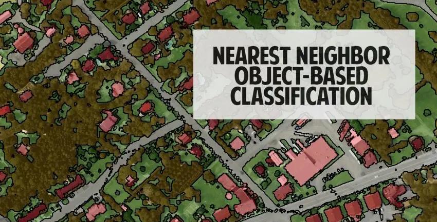
Nearest Neighbor Classification (NN) in eCognition
By the end of this post, you will create a better land cover classification. All because you learned the highly effective nearest neighbor technique in object-based image analysis.
Or you might just learn something neat that we are going to see a lot more of in the future.
We’ve already compared unsupervised, supervised, and object-based classification.
Nearest Neighbor classification is a hidden gem in object-based classification. Almost under the radar, there is nothing that comes close to its capability to classify high spatial resolution remotely sensed data.
Sounds pretty cool? It is.
What is Nearest Neighbor Classification?
Object-based nearest neighbor classification (NN classification) is a super-powered supervised classification technique.
The reason is that you have the advantage of using intelligent image objects with multiresolution segmentation in combination with supervised classification.
What is multiresolution segmentation?
Multiresolution segmentation (MRS) does the digitizing for you. Humans naturally aggregate spatial information into groups. Similarly, it finds logical objects in your image and vectorizes the image. For example, MRS produces thin and long objects for roads. For buildings, it creates square objects of varying scales.
Kind of like this…
You can’t get this using a pixel-by-pixel approach…
Nearest Neighbor Classification Example
The nearest neighbor classification allows you to select samples for each land cover class. You define the criteria (statistics) for classification and the software classifies the remainder of the image.
Nearest Neighbor Classification = Multiresolution Segmentation + Supervised Classification
Now, that we have an overview. Let’s get into the details of the nearest neighbor classification example.
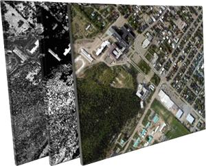
This example uses the following bands: red, green, blue, LiDAR canopy height model (CHM), and LiDAR light intensity (INT).
Step 1. Perform multiresolution segmentation
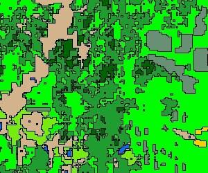
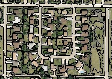
Humans naturally aggregate spatial information into groups. When you see the salt-and-pepper effect in land cover, it’s probably because it uses a pixel-based classification.
Multi-resolution segmentation is why object-based image analysis has emerged for classifying high spatial resolution data sets. MRS creates objects into homogeneous, smart vector polygons.
We can see roads, buildings, grass, and trees as smart objects after multiresolution segmentation. This is why multiresolution segmentation has more value than classifying pixel-by-pixel.
Action: In the process tree, add the multiresolution segmentation algorithm. (Right-click process tree window > Append new > Select multiresolution segmentation algorithm)
This example uses the following criteria:
- SCALE: 100
- SHAPE: 0.1
- COMPACTNESS: 0.5
ACTION: Execute the segmentation. (In the Process Tree window > Right-click multiresolution segmentation algorithm > Click execute)
SCALE: Sets the spatial resolution of the multiresolution segmentation. A higher value will create larger objects.
SHAPE: A higher shape criterion value means that less value will be placed on color during segmentation.
COMPACTNESS: A higher compactness criterion value means the more bound objects will be after segmentation.
The best advice here is trial and error. Experiment with scale, shape, and compactness to get ideal image objects. As a rule of thumb, you want to produce image objects at the biggest possible scale, but still be able to discern between objects.
Step 2. Select training areas
Now, let’s “train” the software by assigning classes to objects. The idea is that these samples will be used to classify the entire image.
But what do we want to classify? What are the land cover classes?
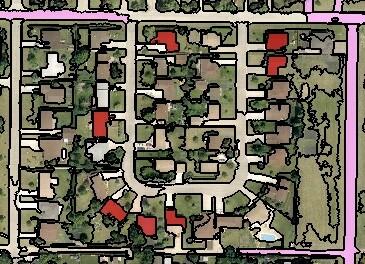
ACTION: In the class hierarchy window, create classes for buildings (red), grass (green), paved surfaces (pink) and treed (brown). (Right-click class hierarchy window > Insert class > Change class name > Click OK)
ACTION: Let’s select samples in the segmented image. Add the “samples” toolbar (View>Toolbars) Select the class and double-click objects to add samples to the training set.
Once you feel that you have a well-represented number of samples for each class, we can now define our statistics.
Note, that we can always return to this step and add more samples after.
Step 3. Define statistics
We now have selected our samples for each land cover class. What statistics are we going to use to classify all the objects in the image?
Defining statistics means adding statistics to the standard NN feature space
ACTION: Open the Edit Standard NN window. (Classification > Nearest Neighbor > Edit Standard NN).
This example uses red, green, blue, LiDAR canopy height model (CHM), and LiDAR light intensity (int) bands. This takes a bit of experimenting to find the right statistics to use. This example uses the statistics below:
Standard NN Feature Space:
- Mean CHM (average LiDAR height in object)
- Standard deviation (height variation in object)
- Mean int (average LiDAR intensity in object)
- Mean red (average red value in object)
Step 4. Classify
- ACTION: In the class hierarchy; add the “standard nearest neighbor” to each class. (Right-click class> Edit > Right-click [and min] > Insert new expression > Standard nearest neighbor)
- ACTION: In the process tree, add the “classification” algorithm. (Right-click process tree > Append New > Select classification algorithm)
- ACTION: Select each class as active and press execute. (In parameter window > checkmark all classes > Right click classification algorithm in process tree > execute)
The classification process will classify all objects in the entire image based on the selected samples and the defined statistics. It will classify each object based on its closeness to the training set.
If you are unhappy with the nearest neighbor classification final product, there are still a couple of options to improve the accuracy.
Here is a list of options to improve your classification:
- Add more samples to the training set.
- Define different statistics.
- Experiment with different scales and criteria in MRS.
- If possible, add more bands (NIR, etc).
You want to automate as much as possible using steps 1-4 with the highest accuracy. But there’s still hope if you didn’t get things right.
Step 5. Object based image editing
Your goal was 100% accuracy, but you’ve only made it to 80% accuracy. That’s really not too bad. You deserve a pat on the back.
If you look for perfection, you’ll never be happy. That’s why the manual editing toolbar exists in eCognition. (View>Toolbars>Manual Editing)
Select the class. Select the object. You have just made a manual edit.
5 easy steps to nearest neighbor classification:
- Perform multiresolution segmentation
- Select training areas
- Define statistics
- Classify
- Manual editing
Take OBIA for a Test-Drive
Nearest neighbor classification is a powerful (and little known) approach to creating a land cover classification.
It’s unique in that you generate smart objects with multiresolution segmentation and supervised classification with the sample editor.
But it does take a bit of practice. It’s an art and science to create a land cover masterpiece.
Master this nearest neighbor classification guide and you are one step closer to becoming an object-based image analysis expert.
Object based image analysis software: