
基于PostGIS的高级应用(4)– 空间查询
目录
一 空间关系
数据库中判定数据之间的关系,使用的是比较操作符,如下:
| 操作符 | 描述 |
|---|---|
| 小于 | |
| > | 大于 |
| 小于等于 | |
| >= | 大于等于 |
| = | 等于 |
| 或!= | 不等于 |
但是在空间数据库中,由于空间数据的多维属性及其不同的几何特征,其判定关系与数值型字符型这些常用数据有非常大的概念性差异。对于GIS来说,空间数据库是核心,GIS开发人员对常用的基于sql比较操作符查询关系表的方式叫“属性查询”,对基于图形空间关系的判定查询叫“空间查询”。所以在说空间查询时,一定要写理清什么是空间关系。
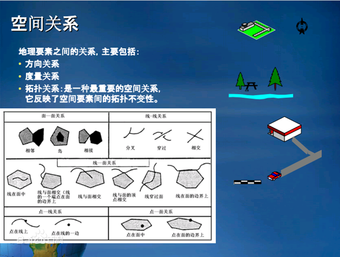
任何涉及地理位置的数据,都具备如下关系:
| 空间关系 | 描述 |
|---|---|
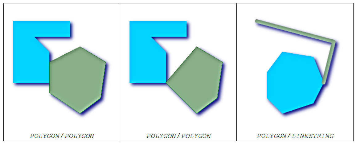
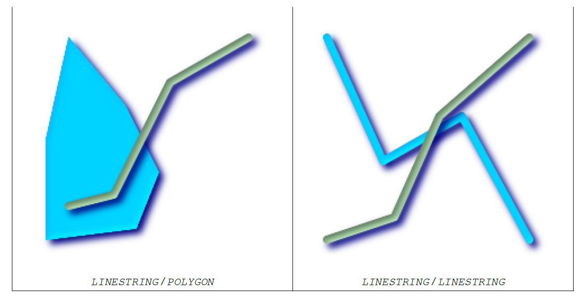
| ST_Intersects | 相交关系,两个图形之间存在公共部分,比如公共点,公共线,公共面 |
| ST_Disjoint | 相离关系,两个图形无丝毫公共部分,与ST_Intersects完全相反 |
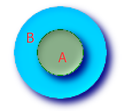
| ST_Contains | 包含关系,图形A包含图形B:ST_Contains(A,B),如点在面内,线在面内。 |
| ST_Within | 被包含关系,图形A被B包含:ST_Within(A,B),与ST_Contains完全相反。 |
| ST_Covers | 覆盖关系,图形A完全覆盖住了图形B:ST_Covers (A,B),部分关系与ST_Contains重叠,但不是完全一样。 |
| ST_Crosses | 穿越关系,图形A与图形B有一部分公共内点,但不是全部。 |
| ST_Equals | 相等关系,两个图形完全相等。 |
| ST_Overlaps | 压盖关系 |
| ST_Touches | 相连关系,两个图形只有边界存在公共连接关系。 |

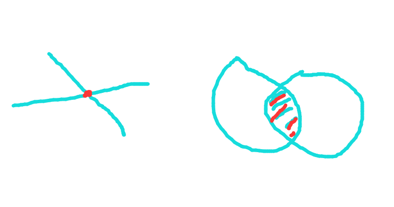
空间关系并非非此即彼的关系,不同空间关系之间肯能存在重叠部分,但又有些许差异,具体需要用户在实际应用时体会。实际应用中,St_Intersects是最常用的一个。
更专业解释参考维基百科详情:https://en.wikipedia.org/wiki/DE-9IM
二 分析优化
正如第一节所说,空间关系之间,既可能是完全互斥的,如相离和相交,包含和被包含,又有似乎重叠的关系,如 包含与压盖,相交与相连。实际应用为了解决一个业务场景,可能有很多种空间方法可以解决问题,但不同的方法之间实际效率需要使用者测试和选择。
2.1 案例说明
某规划公司有两类点数据,一类是公交站点,地铁站点等交通站点数据,数据量约6200条,一类是居民小区房屋点位置数据,数据量约25000条。规划部门希望快速检索站点为中心约200米以外的所有房屋点数据。
房屋测试数据:
--创建房屋测试表
create table house(
    gid serial primary key,
    name text,
    geom geometry(Point,4326)
);
create index house_geom_idx on house using gist(geom);
--插入约25000的测试数据
insert into house(geom) SELECT st_setsrid((ST_Dump(p_geom)).geom,4326)
from (select ST_GeneratePoints(
ST_GeomFromText('Polygon((118.357442 31.231278,119.235188 31.231278,119.235188 32.614617,118.357442 32.614617,118.357442 31.231278))'
), 25000) as p_geom) as b;
站点测试数据:
--创建站点测试表
create table station(
    gid serial primary key,
    name text,
    geom geometry(Point,4326)
);
create index station_geom_idx on station using gist(geom);
--插入测试数据
insert into station(geom) SELECT st_setsrid((ST_Dump(p_geom)).geom,4326)
from (select ST_GeneratePoints(
ST_GeomFromText('Polygon((118.357442 31.231278,119.235188 31.231278,119.235188 32.614617,118.357442 32.614617,118.357442 31.231278))'
), 6200) as p_geom) as b;
创建一个临时的站点缓冲数据表
create table station_buffer(gid serial primary key,geom geometry(Polygon,4326));
create index station_buffer_geom_idx on station_buffer using gist(geom);

insert into station_buffer(geom) select st_buffer(geom,0.002) geom from station;
2.2 空间分析
2.2.1 相离算法
以每个站点为中心,200米为半径,建立缓冲区,合并所有的缓冲区,查询房屋不在这个合并缓冲区范围内的数据,即房屋点与合并缓冲区点相离,这个逻辑是最简单的:
select count(a.*) from house a,(
select st_union(geom) geom from station_buffer
) b where ST_Disjoint(a.geom,b.geom);
但是直接卡死了。。。。
2.2.1 相交反算
另外一个思路是把缓冲区内相交的房屋计算出来,然后根据结果反算不在相交数据集中的数据:
方法一:把缓冲区union成一个大的图形,计算这个图形相交的house,然后反算。
select count(a.*) from house a where gid not in
(select distinct(a.gid) from house a,(select st_union(geom) geom from station_buffer) b where ST_intersects(a.geom,b.geom));
 count
-------
 23434
(1 row)

Time: 17857.083 ms (00:17.857)
方法一虽然花费了17s,但是比直接相离那个逻辑,也是快了不知道几百倍了。。。但还是很卡。
方法二:与方法一基本一致,但是不合并缓冲区。
select count(a.*) from house a where gid not in (
select distinct(a.gid) from house a,station_buffer b where ST_intersects(a.geom,b.geom)
);
 count
-------
 23434
(1 row)

Time: 274.454 ms
方法二直接从16s优化到了274 ms了,质的飞越!
但方法二这里使用了not in,只是为了表达逻辑性的,但not in其实也是很影响性能的,我们试着修改修改看看:
方法三:与方法二一致,只是将not in优化成左连接了。。。
select count(*) from (
select a.*,b.gid as gid2 from house a left join (
select distinct(a.gid) from house a,station_buffer b where ST_intersects(a.geom,b.geom)
) as b on a.gid=b.gid) as c where gid2 is null;
 count
-------
 23434
(1 row)

Time: 62.825 ms
PS:not in可以用not exists和左连接去优化,直接not in是很影响性能的。
我们可以把执行计划贴下:
explain select a.* from house a where gid not in (
select distinct(a.gid) from house a,station_buffer b where ST_intersects(a.geom,b.geom)
);
                                                         QUERY PLAN
----------------------------------------------------------------------------------------------------------------------------
 Seq Scan on house a  (cost=5864.43..6385.93 rows=12500 width=68)
   Filter: (NOT (hashed SubPlan 1))
   SubPlan 1
     ->  Unique  (cost=0.46..5801.93 rows=25000 width=4)
           ->  Gather Merge  (cost=0.46..5692.71 rows=43688 width=4)
                 Workers Planned: 2
                 ->  Nested Loop  (cost=0.43..5237.25 rows=18203 width=4)
                       ->  Parallel Index Scan using house_pkey on house a_1  (cost=0.29..531.05 rows=10417 width=36)
                       ->  Index Scan using station_buffer_geom_idx on station_buffer b  (cost=0.15..0.44 rows=1 width=568)
                             Index Cond: (a_1.geom && geom)
                             Filter: _st_intersects(a_1.geom, geom)
(11 rows)

Time: 1.813 ms
不使用not in:
explain select count(*) from (
select a.*,b.gid as gid2 from house a left join (
select distinct(a.gid) from house a,station_buffer b where ST_intersects(a.geom,b.geom)
) as b on a.gid=b.gid) as c where gid2 is null;
                                                     QUERY PLAN
---------------------------------------------------------------------------------------------------------------------
 Aggregate  (cost=4148.80..4148.81 rows=1 width=8)
   ->  Hash Anti Join  (cost=3741.88..4148.80 rows=1 width=0)
         Hash Cond: (a.gid = a_1.gid)
         ->  Gather  (cost=0.00..313.17 rows=25000 width=4)
               Workers Planned: 2
               ->  Parallel Seq Scan on house a  (cost=0.00..313.17 rows=10417 width=4)
         ->  Hash  (cost=3429.38..3429.38 rows=25000 width=4)
               ->  HashAggregate  (cost=2929.38..3179.38 rows=25000 width=4)
                     Group Key: a_1.gid
                     ->  Gather  (cost=0.28..2820.16 rows=43688 width=4)
                           Workers Planned: 2
                           ->  Nested Loop  (cost=0.28..2820.16 rows=18203 width=4)
                                 ->  Parallel Seq Scan on station_buffer b  (cost=0.00..502.83 rows=2583 width=568)
                                 ->  Index Scan using house_geom_idx on house a_1  (cost=0.28..0.89 rows=1 width=36)
                                       Index Cond: (geom && b.geom)
                                       Filter: _st_intersects(geom, b.geom)
(16 rows)
这个案例的优化,将相离改成了相交,not in改成了左连接,都起到了优化查询案例。
2.3 优化解释
-
相离为什么那么慢?
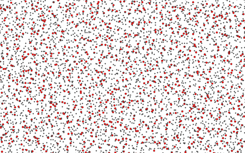 房屋点与红色缓冲区.png
站点200米缓冲区是红色部分,200米是很小的范围,受影响的house是很少的。数据库查询计划,对有索引的,只检索少部分数据才走索引。而相离运算,基本起不到过滤的作用,几乎100%的数据都是相离的,那么会全表查询,全表计算,所以非常卡。
-
为什么union缓冲区这么慢?
相交反算的方法一,把缓冲区合并了一个图形,通过上图可知,红色的缓冲区几乎各个地方都有,合并后的图形的extent(外接矩形)基本是全局的,而无效部分非常大(红色区域之间都是无效部分),gist索引,首先也还是根据这个外接矩形去筛选的。实际应用中,对图形的extent中,无效面积过大的,反而还要去切割去优化io和扫描放大。
具体参考德哥的:
《PostgreSQL 空间st_contains,st_within空间包含搜索优化 – 降IO和降CPU(bound box) (多边形GiST优化)》
《PostgreSQL 空间切割(st_split, ST_Subdivide)功能扩展 – 空间对象网格化 (多边形GiST优化)》
在空间分析中,合理使用gist索引,图形越简单,图形面积占外接矩形面积越大,检索效果越好。反之,这种union图形,图形变复杂,extent变大,图形面积占外接矩形面积越小,效果越差。 -
为啥不使用not in?
这个是sql优化中常用的,使用not exists和左连接,的确起到了优化作用。(案例中gid是主键,有索引)。
空间查询在PostGIS中,也是sql查询,各种优化需要根据实际情况,如分割复杂图形,减少gist索引无效面积,合理使用空间分析的匹配关系,虽然很多逻辑都对,但是高效还是要开发者根据实际情况去调测的,另外其他基本的sql优化也是通用的。本文作者,水平一般般,但是稍微学了点皮毛就尝试了下,验证了一句话:“实践是检验真理的唯一标准”。

